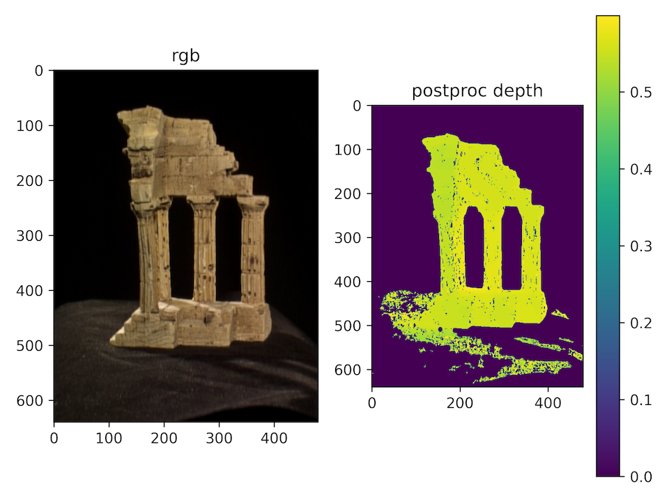
3D Dense Reconstruction
3D Dense Reconstruction from Two View Stereo and MVS (Multi-View Stereo/Plane-Sweep Stereo) Algorithms.
Two-View Stereo
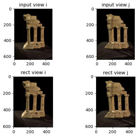
Rectify Two View:
-
Given the pose of each camera, we are first able to compute the right to left transformation \(R_r^l\), \(T_r^l\) and baseline \(b\) of a single pair of images.
-
The rectification rotation matrix \(R_l^{rect}\) to transform the coordinates in the left view to the rectified coordinate frame of left view is computed. The calculation is from the relationship of moving the epipole to the x infinity using: \([1, 0, 0]^T = R_l^{rect} e_l\). The right view rectification rotation matrix will be: \(R_r^{rect} = R_l^{rect} R_r^l\).
-
Compute the homography and warp the image for two views from the relation: \(K_{corr}^{-1} [u_{rect}, v_{rect}, 1]^T = R^{rect} K^{-1} [u, v, 1]^T\)
Disparity Map:
-
Disparity stereo equation:
\[d = \dfrac{fb}{z} = (u_l - c_{xl}) - (u_r - c_{xr})\]where \(c\) denotes the image center, \(z\) is the depth, \(f\) is focal length and \(u\) is pixel coordinates in x direction.
-
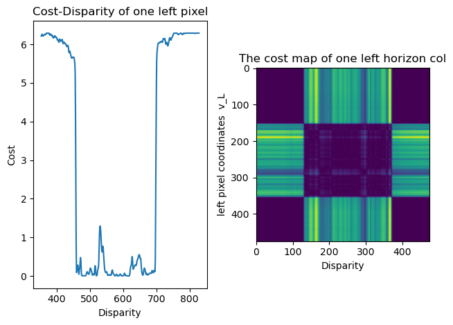
Patchification and Correspondences Matching: Both view are first patchified in to \(3 \times 3\) tiles and correspondences are evaluated on these image tiles with
\[\text{Sum of Squared Difference (SSD)}: SSD = \sum_{(u, v) \in \mathcal{N}} (H(u, v) - F(u, v))^2\] \[\text{Sum of Absolute Differences (SAD)}: SAD = \sum_{(u, v) \in \mathcal{N}} |H(u, v) - F(u, v)|\] \[\text{Zero-mean Normalized Cross Correlation (ZNCC)}: ZNCC = \dfrac{\sum_{(u, v) \in \mathcal{N}} (H(u, v) - \mu_H)(F(u, v) - \mu_F)}{\sqrt{\sum_{(u, v) \in \mathcal{N}}(H(u, v) - \mu_H)^2}\sqrt{\sum_{(u, v) \in \mathcal{N}}(F(u, v) - \mu_F)^2}}\]SSD,SADorZNCCphotometric kernel metrics. Since both views are rectified, according to epipolar constraints, correspondences are bound to be on the same row of pixels.where \(\mathcal{N}\) is all the pixel coordinates in the patch (assume patch \(H\) and \(F\) with the same size). The map of
SSDdisparity candidate cost of one sampling pixel and one sampling row is shown below:
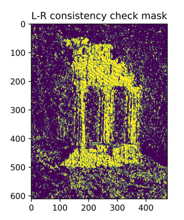
- L-R Consistency: When we found the best right matched patch for each left patch, the match must also be consistent with the result from the other direction. This step is for:
1)Roughly filter out the textureless background.2)Filter out the occuluded pixels only visible in one view. The generated L-R consistency mask is used for postprocessing.
Depth Map and Triangulation:
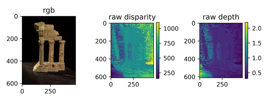
- Raw Disparity & Depth Map: The raw depth is calculated at each pixel with disparity stereo equation from disparity map
- Triangulation: With the calculated depth, all pixels are back projected to point cloud in camera frame.
Postprocessing and Multi-Pair Aggregation:
- Postprocessing: Filtering with L-R consistency mask, background removal, depth cropping, pointcloud outliers removal…
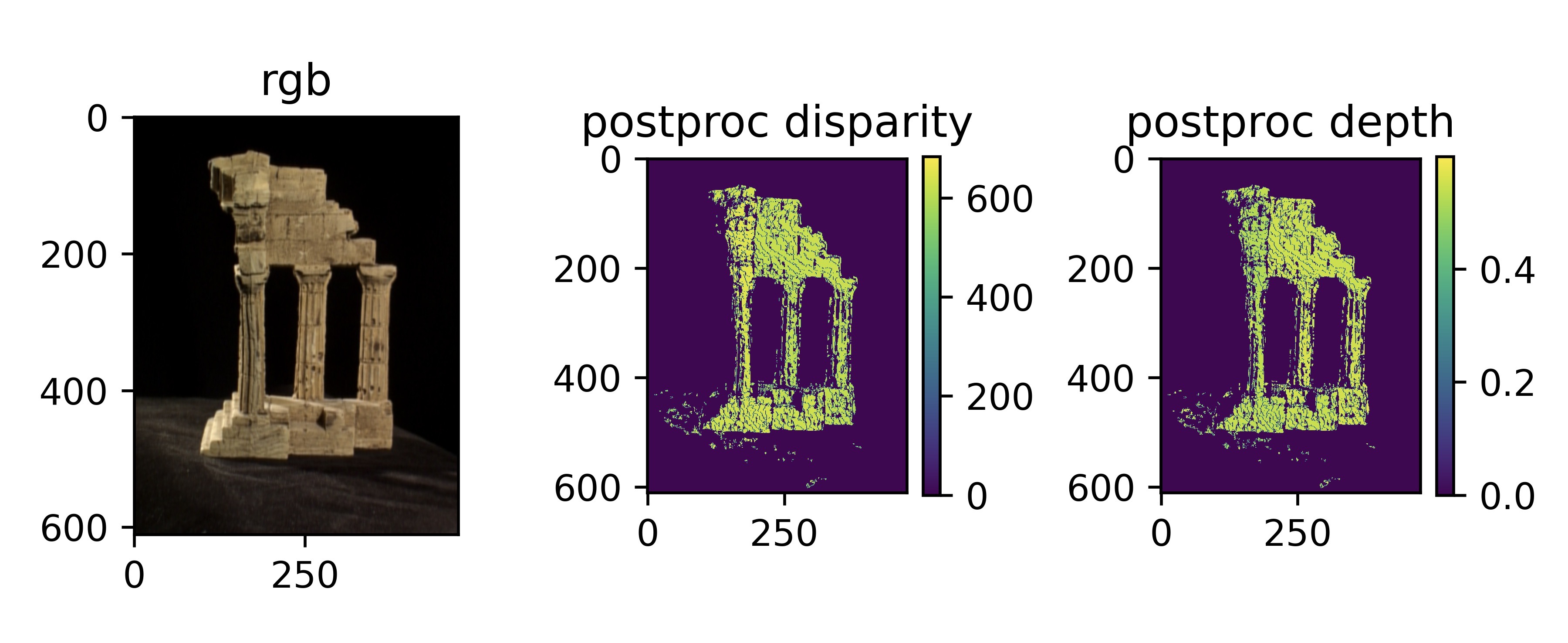
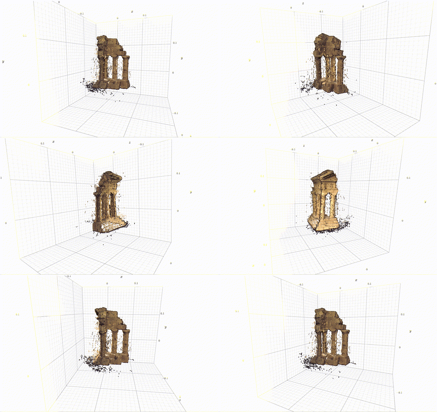
- Multi-pair Aggregation: Several view pairs for two view stereo are performed and the reconstructed point cloud are directly aggregated in the world frame.
Result:
Multiview Stereo/Plane-sweep Stereo
Warping Neighboring Views:
The idea is to sweep a series of imaginary depth planes fronto-parallel with the reference view across a range of candidate depths and project neighboring views onto the imaginary depth plane and back onto the reference view via a computed collineation(Homography). Here number of views \(n=5\) and the middle view is taken as the reference view being warped to.
Disparity Space Image:
For a given image point \((u, v)\) and for discrete depth hypotheses \(d\), the aggregated photometric error \(C(u, v, d)\) with respect to the reference image \(I_R\) can be stored in a volumetric 3D grid called the Disparity Space Image (DSI), where each voxel has value:
where \(\mathcal{N}\) is the set of neighboring images of the reference image, \(I_k(u', v', d)\) is the matched patch in the \(k\)-th image centered on the pixel \((u', v')\) corresponding to the patch \(I_R(u, v)\) in the reference image and depth hypothesis \(d\). \(\rho(\cdot)\) is photometric loss (SSD, SAD, ZNCC…).
The goal is to find a depth function \(d(u, v)\) such that minimize photometric loss and smooth surface.
\[E(d) = E_d(d) + \lambda E_s(d)\]where \(E_d(d)\) is the photometric error and \(E_s(d)\) is the regularization term for depth surface smoothness.
\[E_d(d) = \sum_{(u, v)} C(u, v, d(u, v))\] \[E_s(d) = \sum_{(u, v)} \left( \dfrac{\partial{d(u, v)}}{\partial{u}}\right)^2 + \left(\dfrac{\partial{d(u, v)}}{\partial{v}}\right)^2\]Results:
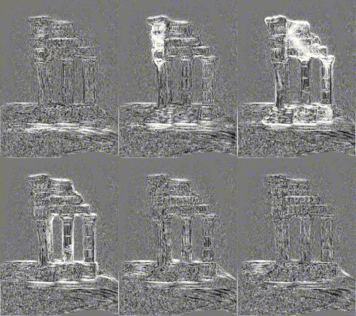
- Depth Candidates Sweeping: When a range of candidate depths are sweeping acoss the Disparity Space Image, bright areas indicate high similarities between matched patches at current depth.
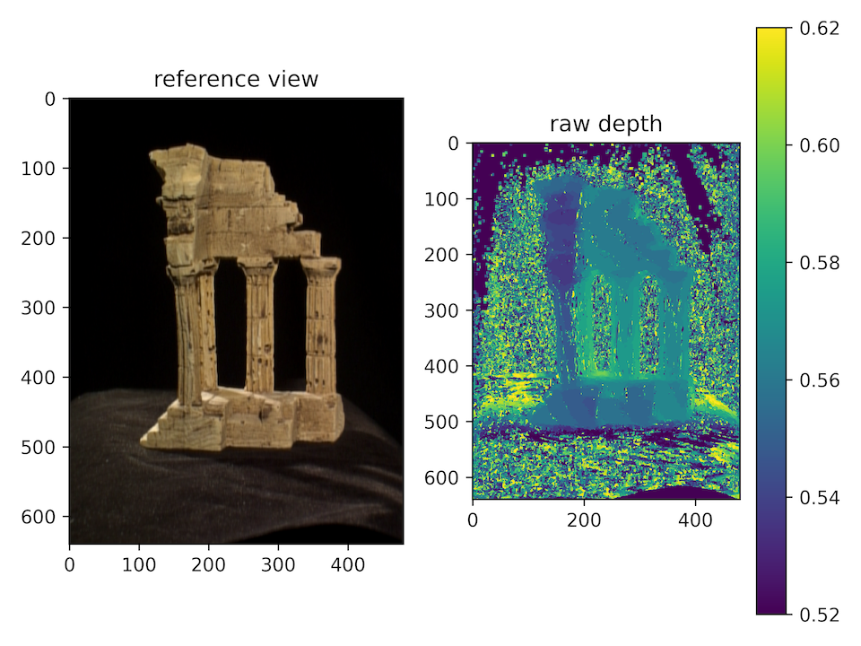
- Raw Depth Map:
- Postprocessed Depth Map:
